Schrödinger's Equation with Python and Numpy

2021-08-26

The Schrödinger Equation
Discretisation
Crank-Nicolson Method
1-Dimensional Simulation
- Confined particle
What Else?

The Schrödinger Equation

We start out with the equation which tells us how our state will change in time ( $\frac{\partial}{\partial t}\ket{\psi}$ ), given its energy ( $\hat H \ket{\psi}$ ):

\begin{equation*} i\hbar\frac{\partial}{\partial t}\ket{\psi} = \hat H \ket{\psi} \end{equation*}

For a single particle system of mass $m$ , we can use the Hamiltonian

\begin{align*} \hat H &= \hat T + \hat V \\ &= -\frac{\hbar^{2}}{2m}\frac{\partial^{2}}{\partial x^{2}} + \hat V \end{align*}

Cool. How do we put this on the computer?

Discretisation

We want to be able to write an equation:

\begin{equation*} \ket{\psi_{t+1}} = \hat M \ket{\psi_{t}} \end{equation*}

Where $\hat M$ is some matrix which tells us: if our state looks like $\ket{\psi_{t}}$ at time $t$ what it'll look like at time $t+1$ . We get the state at time $t+1$ by applying $\hat M$ to our state at time $t$ .

First Derivative

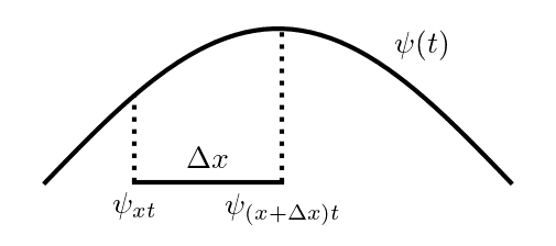
Lets start by splitting up the partial derivative with respect to time ( $\frac{\partial}{\partial t}$ ): Since a derivative is the difference in a function over two closely spaced points, divided by that difference, we can do:

\begin{equation*} \frac{\partial}{\partial t} \ket{\psi_{t}} = \lim_{\Delta t \rightarrow 0} \frac{\ket{\psi_{t+\Delta t}} - \ket{\psi_{t}}}{\Delta t} \end{equation*}

One interesting thing to note here is the choice of going from $t\rightarrow t+\Delta t$ to get the value of the derivative at $t$ . We should hopefully be able to choose any two points in $\left\{\left( t-\alpha\Delta t, t+(1-\alpha)\Delta t \right) \mid \forall \alpha \in \left(0, 1\right)\right\}$ , and this will give the same answer as $\Delta t \rightarrow 0$ , but you can get some nasty functions that don't share this behaviour (eg. the Weierstrass function). Make sure you're dealing with a smooth one :^).

Second Derivative

We'll deal with the second derivative in $x$ in a similar way to the first derivative in $t$ . First, work out the first derivative at the points $x-\frac{\Delta x}{2}$ and $x+\frac{\Delta x}{2}$ , then calculate the derivative between these.

\begin{align*} \frac{\partial^{2}}{\partial x^{2}}\ket{\psi_{x}} &= \lim_{\Delta x \rightarrow 0} \frac{\frac{\partial}{\partial x}\ket{\psi_{x+\frac{\Delta x}{2}}} - \frac{\partial}{\partial x}\ket{\psi_{x-\frac{\Delta x}{2}}}}{\Delta x} \\ &= \lim_{\Delta x \rightarrow 0} \frac{\frac{\ket{\psi_{x+\Delta x}} - \ket{\psi_{x}}}{\Delta x} - \frac{\ket{\psi_x} - \ket{\psi_{x-\Delta x}}}{\Delta x}}{\Delta x} \\ &= \lim_{\Delta x \rightarrow 0} \frac{\ket{\psi_{x+\Delta x}} + \ket{\psi_{x-\Delta x}} - 2\ket{\psi_{x}}}{\Delta x^2} \end{align*}

Getting an equation out of it

We've got discretised versions of the two derivative operators, so we're close to just plugging them into the Schrödinger equation but first those pesky limits need to go.

Removing the limits

Since we're on a computer with finite memory there's no way we can approach $\lim_{\alpha\rightarrow 0}$ , so we need to just choose a small enough value for our differential distances $\Delta \alpha$ . This size can be tuned when we actually come to run the simulations. We want a value small enough that if we decrease it the results of the simulation don't change appreciably, but large enough that the simulations don't take forever or run out of space.

Substitution

After substitution for the derivatives, the Schrödinger equation becomes (now explicitly looking at the components of $\ket{\psi}=\int \mathrm{d}t \mathrm{d}x \psi(x, t)\ket{x, t}$ ):

\begin{align*} i\hbar \frac{\psi(x, t+\Delta t) - \psi(x, t)}{\Delta t} &= -\frac{\hbar^{2}}{2m}\frac{\psi(x+\Delta x, t) + \psi(x - \Delta x, t) - 2\psi(x, t)}{\Delta x^{2}}\\ &+ V(x, t)\psi(x, t) \\ \psi(x, t+\Delta t) &= \psi(x, t) \\ &+ \frac{i\Delta t}{\hbar}\frac{\hbar^{2}}{2m}\frac{\psi(x+\Delta x, t) + \psi(x - \Delta x, t) - 2\psi(x, t)}{\Delta x^{2}} \\&- \frac{i\Delta t}{\hbar}V(x, t)\psi(x, t) \end{align*}

Letting $\alpha = \frac{\hbar \Delta t}{2m \Delta x^{2}}$ , we can get it into a more recognisable matrix equation form:

\begin{align*} \psi(x, t+\Delta t) &= i\alpha \psi(x-\Delta x, t)\\ &+\left(1 + 2i\alpha -\frac{i\Delta t}{\hbar}V(x, t)\right)\psi(x, t) + i\alpha \psi(x+\Delta x, t) \\ &= \Big( \begin{matrix} i\alpha & (1 + 2i\alpha -\frac{i\Delta t}{\hbar}V(x, t)) & i\alpha \end{matrix} \Big) \begin{pmatrix} \psi(x-\Delta x, t) \\ \psi(x, t) \\ \psi(x + \Delta x, t) \end{pmatrix} \end{align*}

We can see that the state $\psi(x, t + \Delta t)$ at $x$ in the next timestep depends on the state of that point in the previous timestep, and the two points at $x-\Delta x$ and $x + \Delta x$ . If we discretise the state, so that instead of having continuous values over a continuous basis of positions, it becomes a sum over points separated by $\Delta x$ :

\begin{equation*} \int \mathrm{d}x \psi(x, t) \ket{x} \rightarrow \sum_{x} \psi_{xt} \ket{x} \end{equation*}

Finally, we can write out the full matrix equation (letting $V'_{xt}=1+2i\alpha-\frac{i\Delta t}{\hbar}V_{xt}$ ):

\begin{align*} \begin{pmatrix} \vdots \\ \psi_{x(t+\Delta t)} \\ \vdots \end{pmatrix} &= \begin{pmatrix} &&\dots \\ \dots & i\alpha & V'_{(x-\Delta x)t} & i\alpha & 0 &\dots \\ \dots & 0&i\alpha & V'_{xt} & i\alpha & \dots \\ \dots & & \dots \end{pmatrix} \begin{pmatrix} \vdots \\ \psi_{(x-2\Delta x)t} \\ \psi_{(x-\Delta x)t} \\ \psi_{xt} \\ \psi_{(x + \Delta x)t} \\ \psi_{(x + 2\Delta x)t} \\ \vdots \end{pmatrix} \\ &= \hat M_t \ket{\psi_t} \end{align*}

Our evolution matrix, which takes us from the state at time $t$ to time $t+\Delta t$ is tri-diagonal. The diagonal depends on the potential and the off-diagonals are all constant.

Crank-Nicolson Method

Our current equation uses the forward Euler method which has some stability problems. If we instead average the value of the Hamiltonian at times $t$ and $t+\Delta t$ we can get a much more stable equation.

\begin{align*} \ket{\psi_{t+\Delta t}} = \frac{1}{2}\left(\hat M_{t}\ket{\psi_{t}} + \hat M_{t+\Delta t}\ket{\psi_{t+\Delta t}}\right) \end{align*}

Rearranging, we've got another equation for $\ket{\psi_{t+\Delta t}}$ :

\begin{align*} \left(I-\frac{1}{2}\hat M_{t+\Delta t}\right)\ket{\psi_{t+\Delta t}} &= \frac{1}{2}\hat M_{t}\ket{\psi_{t}} \\ \ket{\psi_{t+\Delta t}} &= \frac{1}{2}\left(I-\frac{1}{2}\hat M_{t+\Delta t}\right)^{-1}\hat M_{t}\ket{\psi_{t}} \\ &= \hat C \ket{\psi_{t}} \end{align*}

Where $\hat C$ is the Crank-Nicolson matrix.

1-Dimensional Simulation

We've got our equation! Now's time for some code. Our first function will generate the Crank Nicolson matrix, given arguments of: $V_{xt}$ , $V_{x(t+\Delta t)}$ (the potential over positions at that those specific times); $\Delta x$ and $\Delta t$ - the spacing between our coordinates; and $m$ , the mass of the particle.

def crank_nicolson(Δx, Δt, mass, vt1, vt2=None):
    """Generate the Crank-Nicolson matrix that will do our evolution
    vt2 allows us to set a different potential at the next timestep.
    """
    if vt2 is None: vt2 = vt1
    ħ = 1.0545718e-34 # kgm^2/s
    α = ħ*Δt/(2*mass*Δx**2)
    Mt = np.zeros((len(vt1), len(vt1)), dtype=np.complex128)
    off_diag = np.full(len(vt1) - 1, 1j*α, dtype=np.complex128)
    Mt += np.diag(off_diag, 1)
    Mt += np.diag(off_diag, -1)
    Mtdt = np.copy(Mt)
    Mt += np.diag(1 + 2*1j*α - 1j*Δt/ħ*vt1)
    Mtdt += np.diag(1 + 2*1j*α - 1j*Δt/ħ*vt2)
    return 0.5 * np.linalg.inv(np.eye(len(vt1), dtype=np.complex128) - 0.5 * Mtdt) @ Mt

We should also make a function which gets the probability distribution from a state:

def probability(state):
    prob = np.abs(state)**2
    return prob / prob.sum()

And a function which creates a gaussian enveloped state with a given spatial frequency ( $k$ ):

def gaussian(k, σ, x, xs):
    state = np.exp(-(xs-x)**2/(2*σ**2)) * np.exp(1j * k * xs)
    state = state / np.sqrt((np.abs(state)**2).sum())
    return state

Finally, a function which plots a state on a given axis:

def plot_state(xs, state, axis):
    axis.plot(xs, state.real, color="red", label=r"$\mathrm{Re}(\psi)$")
    axis.plot(xs, state.imag, color="blue", label=r"$\mathrm{Im}(\psi)$")
    axis.plot(xs, probability(state), color="black", label=r"$\mathrm{P}(\psi)$")

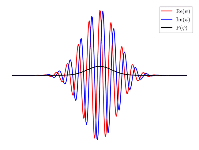
This function plots the real and imaginary parts of the state, and its probability. Lets test it out on a gaussian:

xs = np.linspace(0, 1, 300)
state = gaussian(100, 0.1, 0.5, xs)
fig, axis = plt.subplots()
axis.axis('off')
plot_state(xs, state, axis)
axis.legend()
fig.savefig(filename, dpi=200, bbox_inches="tight")
filename

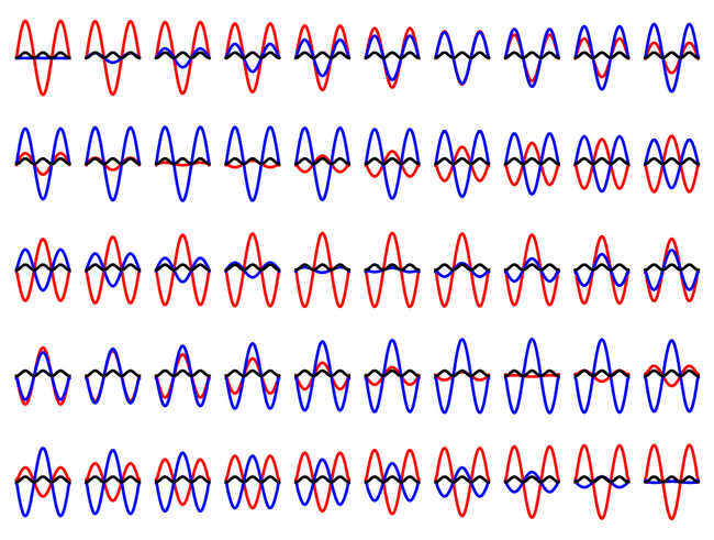
Lets test out the Crank-Nicolson method with an eigenstate of the infinite square well:

xs = np.linspace(0, 1e-32, 100)
state = np.sin(3*xs*np.pi/(1e-32))
state = state / np.sqrt((np.abs(state)**2).sum())
max_val = np.abs(np.max(state)) * 1.2
steps = 31
fig, axs = plt.subplots(5, 10)
C = crank_nicolson(np.abs(xs[1]-xs[0]), 1e-37, 1, np.zeros_like(xs))
C = np.linalg.matrix_power(C, steps)
for i, ax in enumerate(axs.flatten()):
    ax.set_ylim(-max_val, max_val)
    ax.axis('off')
    plot_state(xs, state, ax)
    state = C@state

fig.savefig(filename, dpi=200, bbox_inches="tight")
filename

We can see that the particle stays in the eigenstate, and only the phase of the state changes over the evolution.

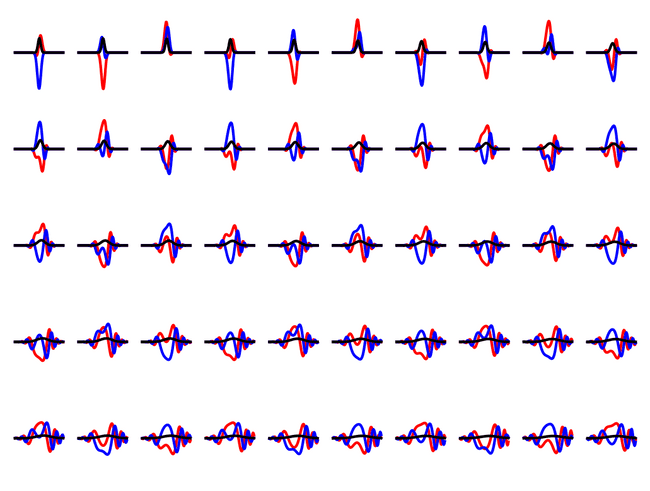
If we instead start with a gaussian state, we can see a much more complicated evolution, with the particle reflecting off the walls.

xs = np.linspace(0, 1e-32, 100)
state = gaussian(1e33, 4e-34, xs[50], xs)
max_val = np.abs(np.max(state)) * 1.2
steps = 1000
fig, axs = plt.subplots(5, 10)
C = crank_nicolson(np.abs(xs[1]-xs[0]), 1e-37, 1, np.zeros_like(xs))
C = np.linalg.matrix_power(C, steps)
for i, ax in enumerate(axs.flatten()):
    ax.set_ylim(-max_val, max_val)
    ax.axis('off')
    plot_state(xs, state, ax)
    state = C@state

fig.savefig(filename, dpi=200, bbox_inches="tight")
filename

We can see the gaussian state disperses into the infinite square well - it's not an eigenstate.

Confined particle

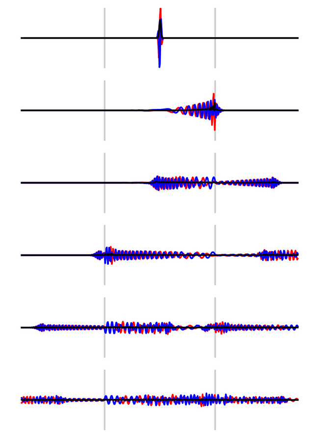
Lets check out what happens if you confine a particle inbetween two finite potential walls.

xs = np.linspace(0, 1e-32, 500)
state = gaussian(5e34, 4e-35, xs[len(xs)//2], xs)
barrier_width = 1
barrier_positions = [150, 350]
potential = np.zeros_like(xs)
potential_value = 36.0
for pos in barrier_positions: potential[pos:pos+barrier_width] = potential_value
fig, axs = plt.subplots(6, 1, figsize=(5, 7))
steps = 2000
max_val = np.abs(np.max(state))
C = crank_nicolson(np.abs(xs[1]-xs[0]), 1e-37, 1, potential)
C = np.linalg.matrix_power(C, steps)
for i, ax in enumerate(axs.flatten()):
    for pos in barrier_positions:
        ax.axvline(xs[pos], color=(0, 0, 0, 0.2))
    ax.set_ylim(-max_val, max_val)
    ax.axis('off')
    plot_state(xs, state, ax)
    state = C@state

fig.savefig(filename, dpi=200, bbox_inches="tight")
filename

The particle bounces between the walls, releasing a small amount of the wavefunction at each barrier.

What Else?

At the moment when the particle hits the boundaries of the space it reflects, but a small change to the Crank-Nicolson matrix could let us simulate cyclic boundary conditions. Physically, this would be like connecting both ends of the simulation space, so the particle's travelling around on a ring. It's also not too big a change to do a 2-dimensional simulation (which may be the subject of a further post??? 🐵)